Generalized Laguerre polynomials

Generalized Laguerre polynomials as computed by orthopolynom.

laguerre(degree, alpha = 0, indeterminate = "x", normalized = FALSE)

Arguments

degree	degree of polynomial
alpha	generalization constant
indeterminate	indeterminate
normalized	provide normalized coefficients

Value

a mpoly object or mpolyList object

See also

orthopolynom::glaguerre.polynomials(), http://en.wikipedia.org/wiki/Laguerre_polynomials

Examples

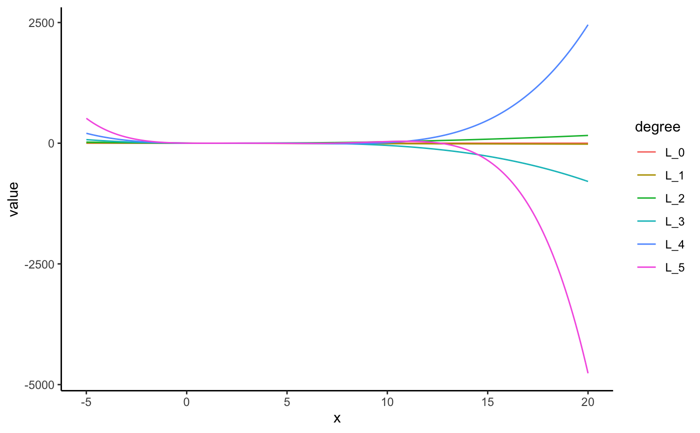
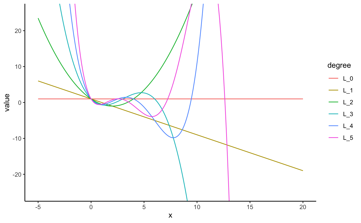
laguerre(0)
#> 1
laguerre(1)
#> 1  -  x
laguerre(2)
#> 1  -  2 x  +  0.5 x^2
laguerre(3)
#> 1  -  3 x  +  1.5 x^2  -  0.1666667 x^3
laguerre(4)
#> 1  -  4 x  +  3 x^2  -  0.6666667 x^3  +  0.04166667 x^4
laguerre(5)
#> 1  -  5 x  +  5 x^2  -  1.666667 x^3  +  0.2083333 x^4  -  0.008333333 x^5
laguerre(6)
#> 1  -  6 x  +  7.5 x^2  -  3.333333 x^3  +  0.625 x^4  -  0.05 x^5  +  0.001388889 x^6

laguerre(2)
#> 1  -  2 x  +  0.5 x^2
laguerre(2, normalized = TRUE)
#> 1  -  2 x  +  0.5 x^2

laguerre(0:5)
#> 1
#> -1 x  +  1
#> 0.5 x^2  -  2 x  +  1
#> -0.1666667 x^3  +  1.5 x^2  -  3 x  +  1
#> 0.04166667 x^4  -  0.6666667 x^3  +  3 x^2  -  4 x  +  1
#> -0.008333333 x^5  +  0.2083333 x^4  -  1.666667 x^3  +  5 x^2  -  5 x  +  1
laguerre(0:5, normalized = TRUE)
#> 1
#> -1 x  +  1
#> 0.5 x^2  -  2 x  +  1
#> -0.1666667 x^3  +  1.5 x^2  -  3 x  +  1
#> 0.04166667 x^4  -  0.6666667 x^3  +  3 x^2  -  4 x  +  1
#> -0.008333333 x^5  +  0.2083333 x^4  -  1.666667 x^3  +  5 x^2  -  5 x  +  1
laguerre(0:5, indeterminate = "t")
#> 1
#> -1 t  +  1
#> 0.5 t^2  -  2 t  +  1
#> -0.1666667 t^3  +  1.5 t^2  -  3 t  +  1
#> 0.04166667 t^4  -  0.6666667 t^3  +  3 t^2  -  4 t  +  1
#> -0.008333333 t^5  +  0.2083333 t^4  -  1.666667 t^3  +  5 t^2  -  5 t  +  1



# visualize the laguerre polynomials

library(ggplot2); theme_set(theme_classic())
library(tidyr)

s <- seq(-5, 20, length.out = 201)
N <- 5 # number of laguerre polynomials to plot
(lagPolys <- laguerre(0:N))
#> 1
#> -1 x  +  1
#> 0.5 x^2  -  2 x  +  1
#> -0.1666667 x^3  +  1.5 x^2  -  3 x  +  1
#> 0.04166667 x^4  -  0.6666667 x^3  +  3 x^2  -  4 x  +  1
#> -0.008333333 x^5  +  0.2083333 x^4  -  1.666667 x^3  +  5 x^2  -  5 x  +  1

# see ?bernstein for a better understanding of
# how the code below works

df <- data.frame(s, as.function(lagPolys)(s))
names(df) <- c("x", paste0("L_", 0:N))
mdf <- gather(df, degree, value, -x)
qplot(x, value, data = mdf, geom = "line", color = degree)

qplot(x, value, data = mdf, geom = "line", color = degree) +
  coord_cartesian(ylim = c(-25, 25))


# laguerre polynomials are orthogonal with respect to the exponential kernel:
L2 <- as.function(laguerre(2))
#> f(.) with . = x
L3 <- as.function(laguerre(3))
#> f(.) with . = x
L4 <- as.function(laguerre(4))
#> f(.) with . = x

w <- dexp
integrate(function(x) L2(x) * L3(x) * w(x), lower = 0, upper = Inf)
#> -5.99989e-07 with absolute error < 5.9e-06
integrate(function(x) L2(x) * L4(x) * w(x), lower = 0, upper = Inf)
#> -1.2e-07 with absolute error < 1.1e-07
integrate(function(x) L3(x) * L4(x) * w(x), lower = 0, upper = Inf)
#> -1.199998e-07 with absolute error < 3e-07