Convert an object to an mpoly

mpoly is the most basic function used to create objects of class mpoly.

as.mpoly(x, ...)

Arguments

x	an object
...	additional arguments to pass to methods

Value

the object formated as a mpoly object.

See also

mp()

Examples

library(ggplot2); theme_set(theme_classic())
#> 
#> Attaching package: ‘ggplot2’
#> The following object is masked from ‘package:mpoly’:
#> 
#>     vars
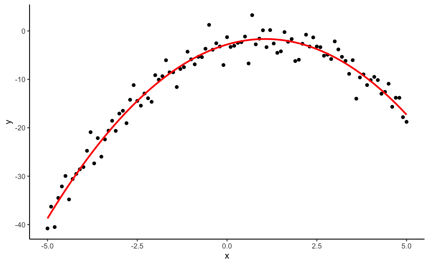
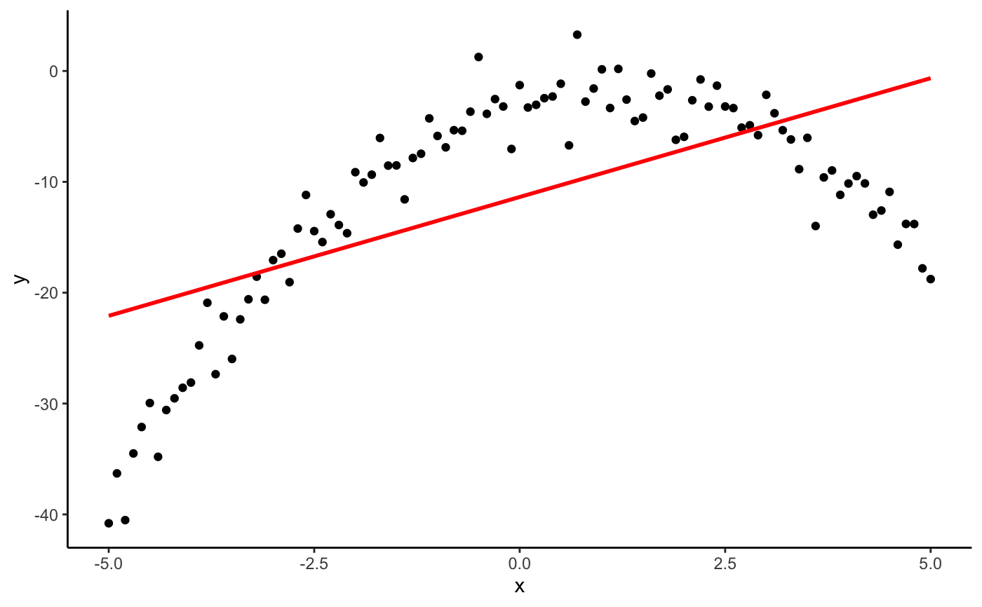
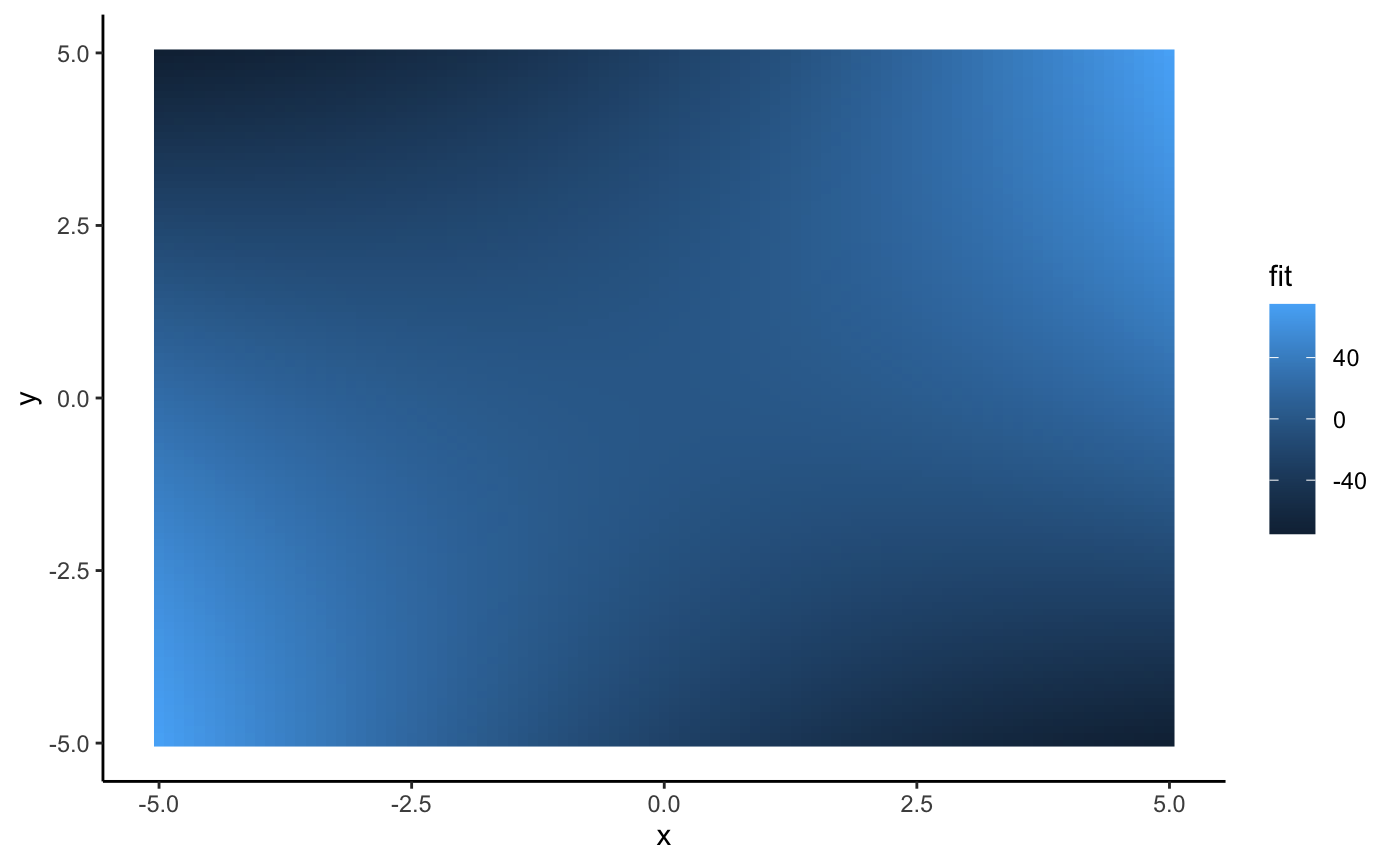
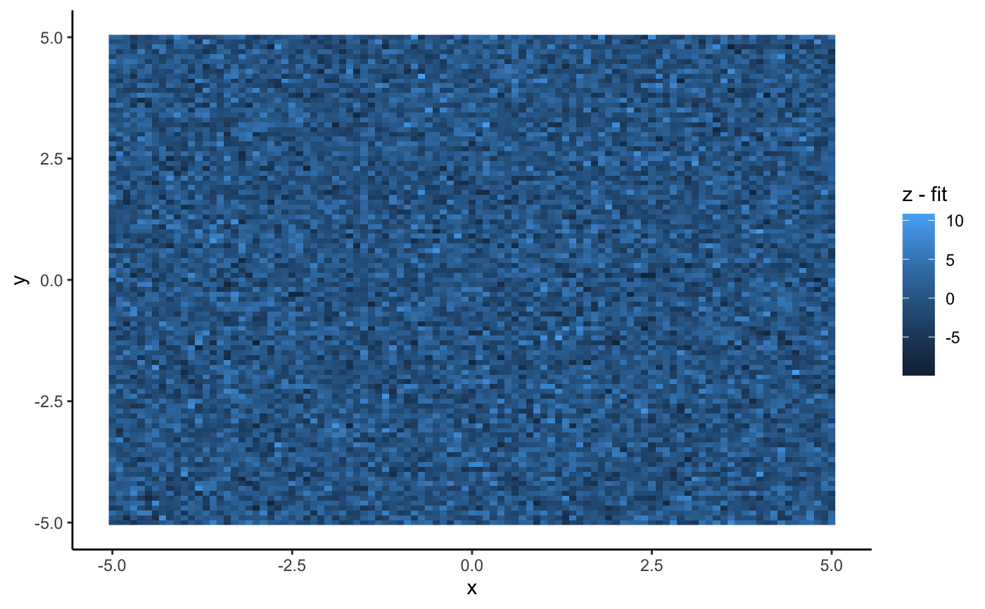
library(dplyr)
#> 
#> Attaching package: ‘dplyr’
#> The following object is masked from ‘package:mpoly’:
#> 
#>     vars
#> The following objects are masked from ‘package:stats’:
#> 
#>     filter, lag
#> The following objects are masked from ‘package:base’:
#> 
#>     intersect, setdiff, setequal, union

n <- 101
s <- seq(-5, 5, length.out = n)



# one dimensional case

df <- data.frame(x = seq(-5, 5, length.out = n)) %>%
  mutate(y = -x^2 + 2*x - 3 + rnorm(n, 0, 2))

(mod <- lm(y ~ x + I(x^2), data = df))
#> 
#> Call:
#> lm(formula = y ~ x + I(x^2), data = df)
#> 
#> Coefficients:
#> (Intercept)            x       I(x^2)  
#>      -2.794        2.144       -1.009  
#> 
(p <- as.mpoly(mod))
#> 2.143584 x  -  1.008662 x^2  -  2.793865
qplot(x, y, data = df) +
  stat_function(fun = as.function(p), colour = "red", size = 1)
#> f(.) with . = x

(mod <- lm(y ~ poly(x, 2, raw = TRUE), data = df))
#> 
#> Call:
#> lm(formula = y ~ poly(x, 2, raw = TRUE), data = df)
#> 
#> Coefficients:
#>             (Intercept)  poly(x, 2, raw = TRUE)1  poly(x, 2, raw = TRUE)2  
#>                  -2.794                    2.144                   -1.009  
#> 
(p <- as.mpoly(mod))
#> 2.143584 x  -  1.008662 x^2  -  2.793865
qplot(x, y, data = df) +
  stat_function(fun = as.function(p), colour = "red", size = 1)
#> f(.) with . = x

(mod <- lm(y ~ poly(x, 1, raw = TRUE), data = df))
#> 
#> Call:
#> lm(formula = y ~ poly(x, 1, raw = TRUE), data = df)
#> 
#> Coefficients:
#>            (Intercept)  poly(x, 1, raw = TRUE)  
#>                -11.367                   2.144  
#> 
(p <- as.mpoly(mod))
#> 2.143584 x  -  11.36749
qplot(x, y, data = df) +
  stat_function(fun = as.function(p), colour = "red", size = 1)
#> f(.) with . = x



# two dimensional case with ggplot2

df <- expand.grid(x = s, y = s) %>%
  mutate(z = x^2 - y^2 + 3*x*y + rnorm(n^2, 0, 3))
qplot(x, y, data = df, geom = "raster", fill = z)

(mod <- lm(z ~ x + y + I(x^2) + I(y^2) + I(x*y), data = df))
#> 
#> Call:
#> lm(formula = z ~ x + y + I(x^2) + I(y^2) + I(x * y), data = df)
#> 
#> Coefficients:
#> (Intercept)            x            y       I(x^2)       I(y^2)     I(x * y)  
#>    0.062597    -0.002988    -0.007926     0.997782    -1.005816     2.995417  
#> 
(mod <- lm(z ~ poly(x, y, degree = 2, raw = TRUE), data = df))
#> 
#> Call:
#> lm(formula = z ~ poly(x, y, degree = 2, raw = TRUE), data = df)
#> 
#> Coefficients:
#>                           (Intercept)  poly(x, y, degree = 2, raw = TRUE)1.0  
#>                              0.062597                              -0.002988  
#> poly(x, y, degree = 2, raw = TRUE)2.0  poly(x, y, degree = 2, raw = TRUE)0.1  
#>                              0.997782                              -0.007926  
#> poly(x, y, degree = 2, raw = TRUE)1.1  poly(x, y, degree = 2, raw = TRUE)0.2  
#>                              2.995417                              -1.005816  
#> 
(p <- as.mpoly(mod))
#> -0.00298808 x  +  0.997782 x^2  -  0.007925533 y  +  2.995417 x y  -  1.005816 y^2  +  0.06259731
df$fit <- apply(df[,c("x","y")], 1, as.function(p))
#> f(.) with . = (x, y)

qplot(x, y, data = df, geom = "raster", fill = fit)

qplot(x, y, data = df, geom = "raster", fill = z - fit) # residuals